Creating Synthetic Magnetic Microscopy Data#
Synthetic data allows for controlled experiments and method validation without the complexity of real-world noise and acquisition artifacts. In this example, we simulate vertical magnetic field maps (Bz) generated by magnetic dipoles embedded in a sample, simulating data from high-resolution magnetic microscopy.
We start with a simple case using a single dipole, then expand to a more complex model with multiple sources.
Why start with one dipole?
Beginning with a single dipole helps isolate and understand the basic shape of the magnetic anomaly, the effect of dipole orientation, and the spatial decay of the magnetic field.
Simulating a Single Dipole#
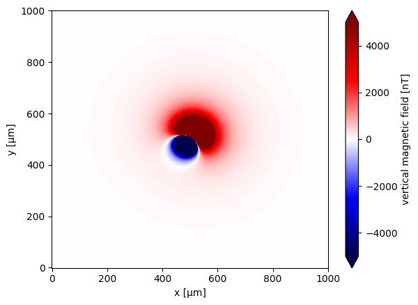
We simulate a single magnetic dipole located at the center of a 1x1 mm area, 15 µm below the sample surface. The observation grid is placed 5 µm above the sample, and the dipole orientation is generated randomly around a mean direction.
Step 1: Import necessary packages#
import numpy as np
import verde as vd
import magali as mg
import harmonica as hm
Step 2: Define grid and simulation parameters#
We define the grid extent, spacing, and the height of the magnetic sensor above the sample.
sensor_sample_distance = 5.0  # µm
region = [0, 1000, 0, 1000]  # µm
spacing = 2  # µm
Step 3: Set the dipole orientation parameters#
We define the mean direction (inclination and declination) of the dipole moment and a small dispersion angle.
true_inclination = 30  # degrees
true_declination = 40  # degrees
true_dispersion_angle = 5  # degrees
size = 1  # only one dipole
Step 4: Generate random dipole orientation#
We use a helper function to generate a random orientation around the true direction.
directions_inclination, directions_declination = mg.random_directions(
    true_inclination,
    true_declination,
    true_dispersion_angle,
    size=size,
    random_state=5,
)
Step 5: Define dipole location and moment#
The dipole is located at the center of the region and placed 15 µm below the surface. Its moment has a small magnitude, pointing in the random direction defined earlier.
dipole_coordinates = (500, 500, -15)  # x, y, z in µm

dipole_moments = hm.magnetic_angles_to_vec(
    inclination=directions_inclination,
    declination=directions_declination,
    intensity=5e-11,  # A·m²
)
Step 6: Simulate the magnetic field#
We now compute the vertical magnetic field (Bz) produced by this single dipole over the defined grid.
data = mg.dipole_bz_grid(
    region, spacing, sensor_sample_distance,
    dipole_coordinates, dipole_moments
)
Step 7: Visualize the results#
The magnetic field is shown using a diverging colormap. Note the characteristic dipolar shape of the field.
data.plot.pcolormesh(cmap="seismic", vmin=-5000, vmax=5000)
<matplotlib.collections.QuadMesh at 0x7f94ecd26ed0>
Simulating a Complex Dipole Distribution#
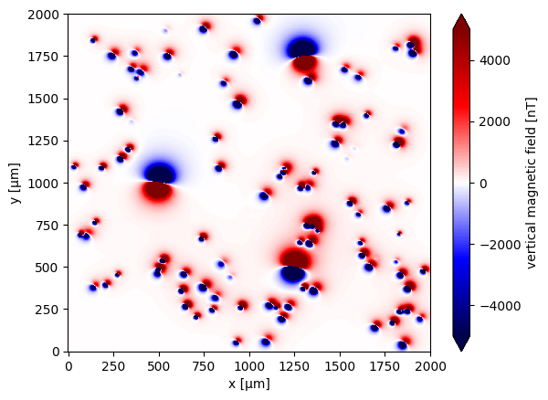
After understanding the basic behavior of a single magnetic source, we can now simulate a more realistic scenario with multiple dipoles. This setup includes dozens of randomly distributed and oriented dipoles, with a few manually placed stronger sources.
We simulate a complex magnetic source model containing 100 randomly oriented dipoles and 3 manually defined dipoles with known properties. The sources are located beneath a 2x2 mm area, and the magnetic field is computed on a dense observation grid 5 µm above the sample.
Step 1: Import necessary packages#
import numpy as np
import verde as vd
import magali as mg
import harmonica as hm
Step 2: Define grid and simulation parameters#
We define a larger simulation region and keep the same grid spacing and sensor-sample distance.
sensor_sample_distance = 5.0  # µm
region = [0, 2000, 0, 2000]  # µm
spacing = 2  # µm
Step 3: Set dipole orientation model#
We define a region on the surface of a sphere centered around a mean direction, with a small dispersion angle.
true_inclination = 30  # degrees
true_declination = 40  # degrees
true_dispersion_angle = 5  # degrees
size = 100  # number of random dipoles
Step 4: Generate dipole directions#
We sample inclination and declination angles from the distribution.
directions_inclination, directions_declination = mg.random_directions(
    true_inclination,
    true_declination,
    true_dispersion_angle,
    size=size,
    random_state=5,
)
Step 5: Define dipole locations and intensities#
Dipoles are randomly positioned within the region. We also manually append three additional dipoles with higher magnetic intensity.
dipoles_amplitude = abs(np.random.normal(0, 100, size)) * 1.0e-14

dipole_coordinates = (
    np.concatenate([np.random.randint(30, 1970, size), [1250, 1300, 500]]),  # x
    np.concatenate([np.random.randint(30, 1970, size), [500, 1750, 1000]]),  # y
    np.concatenate([np.random.randint(-20, -1, size), [-15, -15, -30]]),     # z
)
Step 6: Construct dipole moment vectors#
We combine the random and manual sources into a single set of moment vectors.
dipole_moments = hm.magnetic_angles_to_vec(
    inclination=np.concatenate([directions_inclination, [10, -10, -5]]),
    declination=np.concatenate([directions_declination, [10, 170, 190]]),
    intensity=np.concatenate([dipoles_amplitude, [5e-11, 5e-11, 5e-11]]),
)
Step 7: Simulate the magnetic field#
We calculate the total vertical field (Bz) from all sources at each point on the grid.
data = mg.dipole_bz_grid(
    region, spacing, sensor_sample_distance,
    dipole_coordinates, dipole_moments
)
Step 8: Visualize the results#
The resulting field shows the combined magnetic signal of all sources.
data.plot.pcolormesh(cmap="seismic", vmin=-5000, vmax=5000)
<matplotlib.collections.QuadMesh at 0x7f94eccb3410>