Upward derivative of a regular grid
Note
Click here to download the full example code
Upward derivative of a regular grid
Out:
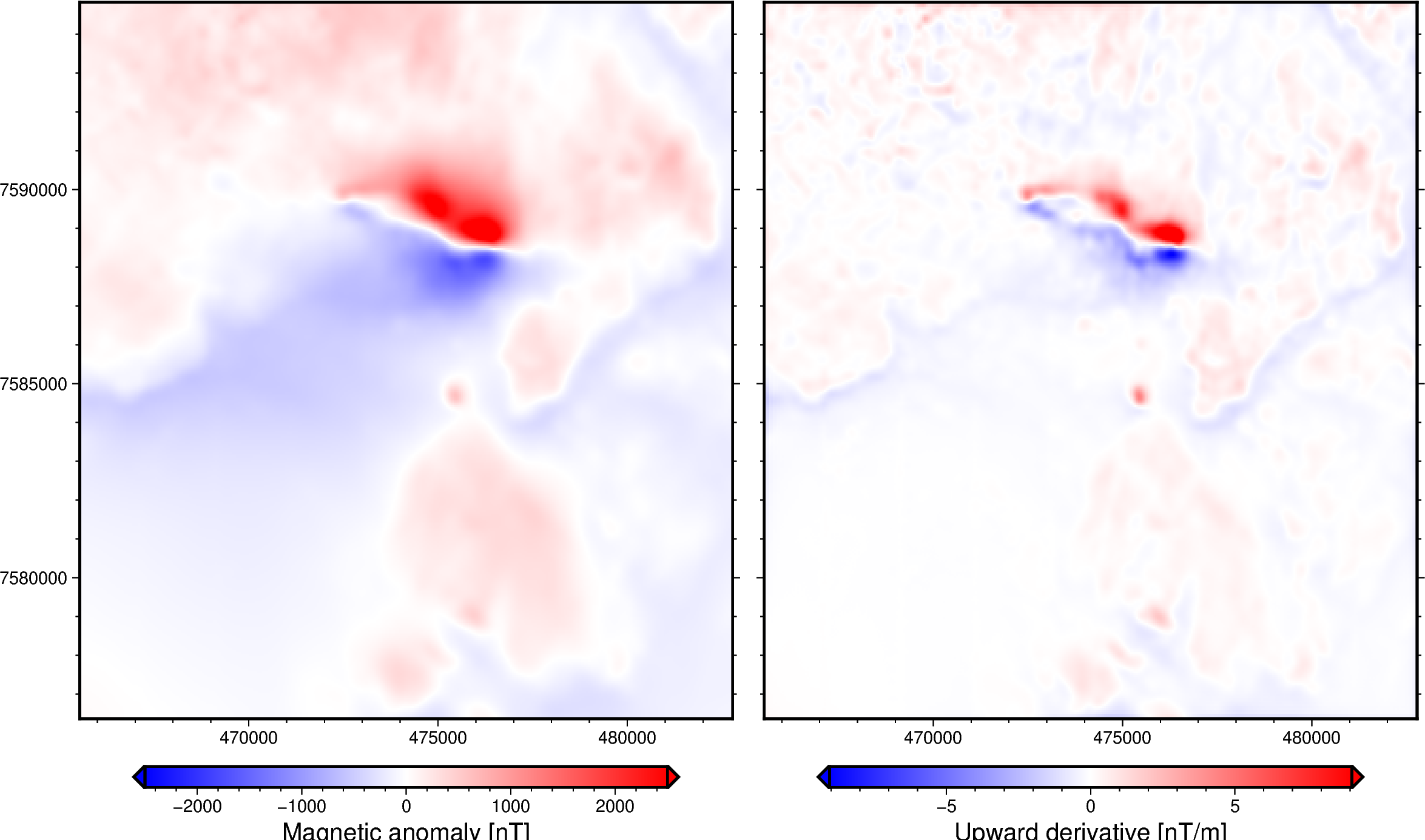
Upward derivative:
 <xarray.DataArray (northing: 370, easting: 346)>
array([[ 0.95819797,  0.62479631,  0.65249329, ..., -1.73446106,
        -1.67664073, -2.7243531 ],
       [ 0.63634155,  0.21904983,  0.23107703, ..., -0.49049877,
        -0.45948262, -1.68410265],
       [ 0.66359221,  0.23536193,  0.2450619 , ..., -0.51034902,
        -0.49225175, -1.75482593],
       ...,
       [ 3.3946594 ,  0.9299787 ,  0.84907987, ..., -0.18739683,
        -0.37947336, -1.13012159],
       [ 3.28895305,  0.89679032,  0.84612464, ..., -0.15550245,
        -0.36489469, -1.12153511],
       [ 5.04819984,  2.91262219,  2.80733139, ...,  0.11714946,
        -0.38706034, -1.26040298]])
Coordinates:
  * northing  (northing) float64 7.576e+06 7.576e+06 ... 7.595e+06 7.595e+06
  * easting   (easting) float64 4.655e+05 4.656e+05 ... 4.827e+05 4.828e+05
<IPython.core.display.Image object>
import ensaio
import pygmt
import verde as vd
import xarray as xr
import xrft

import harmonica as hm

# Fetch magnetic grid over the Lightning Creek Sill Complex, Australia using
# Ensaio and load it with Xarray
fname = ensaio.fetch_lightning_creek_magnetic(version=1)
magnetic_grid = xr.load_dataarray(fname)

# Pad the grid to increase accuracy of the FFT filter
pad_width = {
    "easting": magnetic_grid.easting.size // 3,
    "northing": magnetic_grid.northing.size // 3,
}
# drop the extra height coordinate
magnetic_grid_no_height = magnetic_grid.drop_vars("height")
magnetic_grid_padded = xrft.pad(magnetic_grid_no_height, pad_width)

# Compute the upward derivative of the grid
deriv_upward = hm.derivative_upward(magnetic_grid_padded)

# Unpad the derivative grid
deriv_upward = xrft.unpad(deriv_upward, pad_width)

# Show the upward derivative
print("\nUpward derivative:\n", deriv_upward)


# Plot original magnetic anomaly and the upward derivative
fig = pygmt.Figure()
with fig.subplot(nrows=1, ncols=2, figsize=("28c", "15c"), sharey="l"):
    with fig.set_panel(panel=0):
        # Make colormap of data
        scale = 2500
        pygmt.makecpt(cmap="polar+h", series=[-scale, scale], background=True)
        # Plot magnetic anomaly grid
        fig.grdimage(
            grid=magnetic_grid,
            projection="X?",
            cmap=True,
        )
        # Add colorbar
        fig.colorbar(
            frame='af+l"Magnetic anomaly [nT]"',
            position="JBC+h+o0/1c+e",
        )
    with fig.set_panel(panel=1):
        # Make colormap for upward derivative (saturate it a little bit)
        scale = 0.6 * vd.maxabs(deriv_upward)
        pygmt.makecpt(cmap="polar+h", series=[-scale, scale], background=True)
        # Plot upward derivative
        fig.grdimage(grid=deriv_upward, projection="X?", cmap=True)
        # Add colorbar
        fig.colorbar(
            frame='af+l"Upward derivative [nT/m]"',
            position="JBC+h+o0/1c+e",
        )
fig.show()
Total running time of the script: ( 0 minutes 2.664 seconds)