Upward continuation of a regular grid
Note
Click here to download the full example code
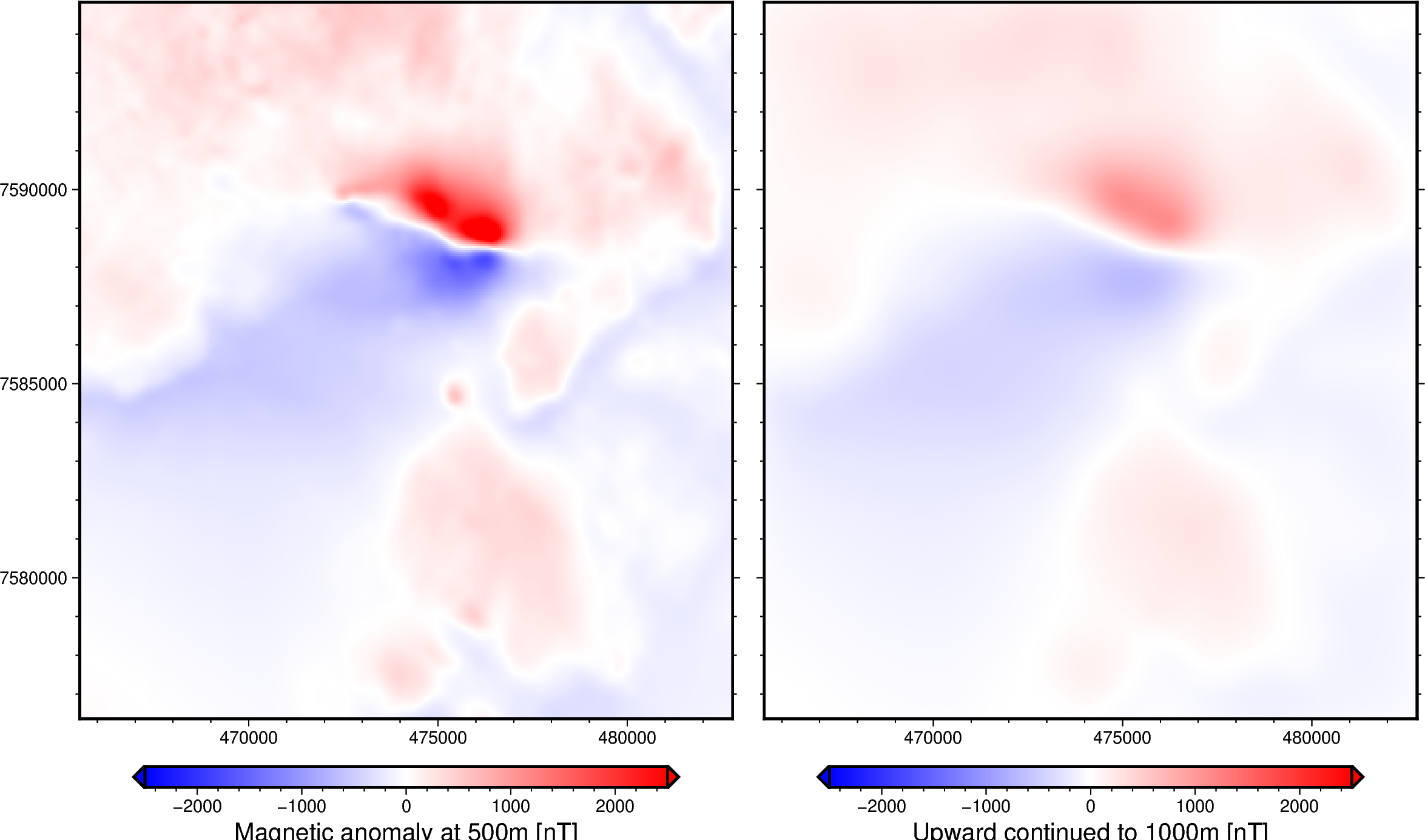
Upward continuation of a regular grid
Out:
Upward continued magnetic grid:
 <xarray.DataArray (northing: 370, easting: 346)>
array([[  1.5318864 ,   1.85100319,   2.13679603, ..., -33.60489015,
        -31.65890937, -29.67750194],
       [  1.82033329,   2.17484726,   2.49236703, ..., -35.96395426,
        -33.83598794, -31.6667934 ],
       [  2.07317532,   2.45927687,   2.80499305, ..., -38.27995984,
        -35.97492132, -33.62307385],
       ...,
       [ 50.44856723,  53.84378576,  57.13892691, ...,   4.05301916,
          2.81272894,   1.764435  ],
       [ 47.56514008,  50.69951642,  53.74614319, ...,   4.66844263,
          3.44420588,   2.39520989],
       [ 44.6368305 ,  47.50470955,  50.29752195, ...,   5.03756138,
          3.86192233,   2.84250804]])
Coordinates:
  * northing  (northing) float64 7.576e+06 7.576e+06 ... 7.595e+06 7.595e+06
  * easting   (easting) float64 4.655e+05 4.656e+05 ... 4.827e+05 4.828e+05
<IPython.core.display.Image object>
import ensaio
import pygmt
import xarray as xr
import xrft

import harmonica as hm

# Fetch magnetic grid over the Lightning Creek Sill Complex, Australia using
# Ensaio and load it with Xarray
fname = ensaio.fetch_lightning_creek_magnetic(version=1)
magnetic_grid = xr.load_dataarray(fname)

# Pad the grid to increase accuracy of the FFT filter
pad_width = {
    "easting": magnetic_grid.easting.size // 3,
    "northing": magnetic_grid.northing.size // 3,
}
# drop the extra height coordinate
magnetic_grid_no_height = magnetic_grid.drop_vars("height")
magnetic_grid_padded = xrft.pad(magnetic_grid_no_height, pad_width)

# Upward continue the magnetic grid, from 500 m to 1000 m
# (a height displacement of 500m)
upward_continued = hm.upward_continuation(magnetic_grid_padded, height_displacement=500)

# Unpad the upward continued grid
upward_continued = xrft.unpad(upward_continued, pad_width)

# Show the upward continued grid
print("\nUpward continued magnetic grid:\n", upward_continued)


# Plot original magnetic anomaly and the upward continued grid
fig = pygmt.Figure()
with fig.subplot(nrows=1, ncols=2, figsize=("28c", "15c"), sharey="l"):
    # Make colormap for both plots data
    scale = 2500
    pygmt.makecpt(cmap="polar+h", series=[-scale, scale], background=True)
    with fig.set_panel(panel=0):
        # Plot magnetic anomaly grid
        fig.grdimage(
            grid=magnetic_grid,
            projection="X?",
            cmap=True,
        )
        # Add colorbar
        fig.colorbar(
            frame='af+l"Magnetic anomaly at 500m [nT]"',
            position="JBC+h+o0/1c+e",
        )
    with fig.set_panel(panel=1):
        # Plot upward continued grid
        fig.grdimage(grid=upward_continued, projection="X?", cmap=True)
        # Add colorbar
        fig.colorbar(
            frame='af+l"Upward continued to 1000m [nT]"',
            position="JBC+h+o0/1c+e",
        )
fig.show()
Total running time of the script: ( 0 minutes 2.616 seconds)