How to use Choclo#
The simplest case#
Using Choclo is very simple, but it requires some work from our side. Let’s say
we need to compute the upward component of the gravitational acceleration that
a single rectangular prism produces on a single computation point. To do so we
can just call the choclo.prism.gravity_u function:
import numpy as np
from choclo.prism import gravity_u

# Define a single computation point
easting, northing, upward = 0.0, 0.0, 10.0

# Define the boundaries of the prism as a list
prism = [-10.0, 10.0, -7.0, 7.0, -15.0, -5.0]

# And its density
density = 400.0

# Compute the upward component of the grav. acceleration
g_u = gravity_u(easting, northing, upward, *prism, density)
g_u
-1.6539652880538094e-07
But this case is very simple: we usually deal with multiple sources and multiple computation points.
Multiple sources and computation points#
In case we have a collection of prisms with certain densities:
prisms = np.array([
    [-10.0, 0.0, -7.0, 0.0, -15.0, -10.0],
    [-10.0, 0.0, 0.0, 7.0, -25.0, -15.0],
    [0.0, 10.0, -7.0, 0.0, -20.0, -13.0],
    [0.0, 10.0, 0.0, 7.0, -12.0, -8.0],
])
densities = np.array([200.0, 300.0, -100.0, 400.0])
And a set of observation points:
easting = np.linspace(-50.0, 50.0, 21)
northing = np.linspace(-40.0, 40.0, 21)
easting, northing = np.meshgrid(easting, northing)
upward = 10 * np.ones_like(easting)

coordinates = (easting.ravel(), northing.ravel(), upward.ravel())
And we want to compute the gravitational acceleration that those prisms generate on each observation point, we need to write some kind of loop that computes the effect of each prism on each observation point and adds it to a running result.
A possible solution would be to use Python for loops:
def gravity_upward_slow(coordinates, prisms, densities):
    """
    Compute the upward component of the acceleration of a set of prisms
    """
    # Unpack coordinates of the observation points
    easting, northing, upward = coordinates[:]
    # Initialize a result array full of zeros
    result = np.zeros_like(easting, dtype=np.float64)
    # Compute the upward component that every prism generate on each
    # observation point
    for i in range(len(easting)):
        for j in range(prisms.shape[0]):
            result[i] += gravity_u(
                easting[i], northing[i], upward[i], *prisms[j, :], densities[j]
            )
    return result
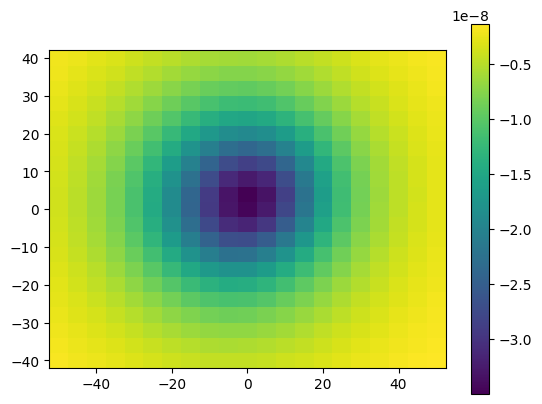
We use this function to compute the field on every point of the grid:
g_u = gravity_upward_slow(coordinates, prisms, densities)
And plot the results:
import matplotlib.pyplot as plt

plt.pcolormesh(easting, northing, g_u.reshape(easting.shape), shading='auto')
plt.gca().set_aspect("equal")
plt.colorbar()
plt.show()
For loops are known to be slow, and in case we are working with very large models and a large number of computation points these calculations could take too long. So this solution is not recommended.
Important
Using Python for loops to run Choclo’s functions is not advisable!
We can write a much faster and efficient solution relying on numba.
Since every function in Choclo is being JIT compiled, we can safely include
calls to these functions inside other JIT compiled functions. So we can write
an alternative function by adding a @numba.jit decorator:
import numba

@numba.jit(nopython=True)
def gravity_upward_jit(coordinates, prisms, densities):
    """
    Compute the upward component of the acceleration of a set of prisms
    """
    # Unpack coordinates of the observation points
    easting, northing, upward = coordinates[:]
    # Initialize a result array full of zeros
    result = np.zeros_like(easting, dtype=np.float64)
    # Compute the upward component that every prism generate on each
    # observation point
    for i in range(len(easting)):
        for j in range(prisms.shape[0]):
            result[i] += gravity_u(
                easting[i],
                northing[i],
                upward[i],
                prisms[j, 0],
                prisms[j, 1],
                prisms[j, 2],
                prisms[j, 3],
                prisms[j, 4],
                prisms[j, 5],
                densities[j],
            )
    return result

g_u = gravity_upward_jit(coordinates, prisms, densities)

plt.pcolormesh(easting, northing, g_u.reshape(easting.shape), shading='auto')
plt.gca().set_aspect("equal")
plt.colorbar()
plt.show()

Let’s benchmark these two functions to see how much faster the decorated function runs:
%timeit gravity_upward_slow(coordinates, prisms, densities)
5.63 ms ± 16.1 μs per loop (mean ± std. dev. of 7 runs, 100 loops each)
%timeit gravity_upward_jit(coordinates, prisms, densities)
462 μs ± 3.11 μs per loop (mean ± std. dev. of 7 runs, 1,000 loops each)
From these numbers we can see that we have significantly reduced the computation time by several factors by just decorating our function.
Note
The benchmarked times may vary if you run them in your system.
See also
Check How to measure the performance of Numba? to learn more about how to properly benchmark jitted functions.
Parallelizing our runs#
We have already shown how we can reduce the computation times of our forward
modelling by decorating our functions with @numba.jit(nopython=True). But
this is just the first step: all the computations were being run in serial in
a single CPU. We can harness the full power of our modern multiprocessors CPUs
by parallelizing our runs. To do so we need to use the numba.prange
instead of the regular Python range function and slightly change the
decorator of our function by adding a parallel=True argument:
@numba.jit(nopython=True, parallel=True)
def gravity_upward_parallel(coordinates, prisms, densities):
    """
    Compute the upward component of the acceleration of a set of prisms
    """
    # Unpack coordinates of the observation points
    easting, northing, upward = coordinates[:]
    # Initialize a result array full of zeros
    result = np.zeros_like(easting, dtype=np.float64)
    # Compute the upward component that every prism generate on each
    # observation point
    for i in numba.prange(len(easting)):
        for j in range(prisms.shape[0]):
            result[i] += gravity_u(
                easting[i],
                northing[i],
                upward[i],
                prisms[j, 0],
                prisms[j, 1],
                prisms[j, 2],
                prisms[j, 3],
                prisms[j, 4],
                prisms[j, 5],
                densities[j],
            )
    return result

g_u = gravity_upward_parallel(coordinates, prisms, densities)

plt.pcolormesh(easting, northing, g_u.reshape(easting.shape), shading='auto')
plt.gca().set_aspect("equal")
plt.colorbar()
plt.show()

With numba.prange we can specify which loop we want to run in parallel.
Since we are updating the values of results on each iteration, it’s
advisable to parallelize the loop over the observation points.
By setting parallel=True in the decorator we are telling Numba to
parallelize this function, otherwise Numba will reinterpret the
numba.prange function as a regular range and run this loop in serial.
Note
In some applications it’s desirable that our forward models are run in
serial. For example, if they are part of larger problem that gets
parallelized at a higher level. The parallel parameter in the
numba.jit decorator allows us to change this behaviour at will without
having to modify the function code.
Let’s benchmark this function against the non-parallelized
gravity_upward_jit:
%timeit gravity_upward_jit(coordinates, prisms, densities)
462 μs ± 4.14 μs per loop (mean ± std. dev. of 7 runs, 1,000 loops each)
%timeit gravity_upward_parallel(coordinates, prisms, densities)
201 μs ± 497 ns per loop (mean ± std. dev. of 7 runs, 10,000 loops each)
By distributing the load between multiple processors we were capable of lowering the computation time by a few more factors.