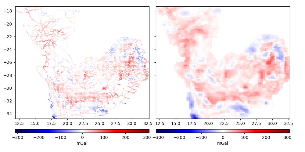
Gridding in spherical coordinates¶

The curvature of the Earth must be taken into account when gridding and processing magnetic or gravity data on large regions. In these cases, projecting the data may introduce errors due to the distortions caused by the projection.

harmonica.EquivalentSourcesSph implements the equivalent sources technique in spherical coordinates. It has the same advantages as the Cartesian equivalent sources (harmonica.EquivalentSources) while taking into account the curvature of the Earth.

Out:

/usr/share/miniconda3/envs/testing/lib/python3.9/site-packages/boule/ellipsoid.py:458: UserWarning: Formulas used are valid for points outside the ellipsoid.Height must be greater than or equal to zero.
  warn(
/usr/share/miniconda3/envs/testing/lib/python3.9/site-packages/sklearn/linear_model/_base.py:148: FutureWarning: 'normalize' was deprecated in version 1.0 and will be removed in 1.2. Please leave the normalize parameter to its default value to silence this warning. The default behavior of this estimator is to not do any normalization. If normalization is needed please use sklearn.preprocessing.StandardScaler instead.
  warnings.warn(
R² score: 0.9999999999915354

Generated grid:
 <xarray.Dataset>
Dimensions:              (spherical_latitude: 88, longitude: 105)
Coordinates:
  * longitude            (longitude) float64 11.91 12.11 12.31 ... 32.48 32.68
  * spherical_latitude   (spherical_latitude) float64 -34.76 -34.56 ... -17.28
    radius               (spherical_latitude, longitude) float64 6.378e+06 .....
Data variables:
    gravity_disturbance  (spherical_latitude, longitude) float64 -0.5771 ... ...
Attributes:
    metadata:  Generated by EquivalentSourcesSph(damping=0.001, relative_dept...

import boule as bl
import matplotlib.pyplot as plt
import numpy as np
import verde as vd

import harmonica as hm

# Fetch the sample gravity data from South Africa
data = hm.datasets.fetch_south_africa_gravity()

# Downsample the data using a blocked mean to speed-up the computations
# for this example. This is preferred over simply discarding points to avoid
# aliasing effects.
blocked_mean = vd.BlockReduce(np.mean, spacing=0.2, drop_coords=False)
(longitude, latitude, elevation), gravity_data = blocked_mean.filter(
    (data.longitude, data.latitude, data.elevation),
    data.gravity,
)

# Compute gravity disturbance by removing the gravity of normal Earth
ellipsoid = bl.WGS84
gamma = ellipsoid.normal_gravity(latitude, height=elevation)
gravity_disturbance = gravity_data - gamma

# Convert data coordinates from geodetic (longitude, latitude, height) to
# spherical (longitude, spherical_latitude, radius).
coordinates = ellipsoid.geodetic_to_spherical(longitude, latitude, elevation)

# Create the equivalent sources
eqs = hm.EquivalentSourcesSph(damping=1e-3, relative_depth=10000)

# Fit the sources coefficients to the observed magnetic anomaly
eqs.fit(coordinates, gravity_disturbance)

# Evaluate the data fit by calculating an R² score against the observed data.
# This is a measure of how well the sources fit the data, NOT how good the
# interpolation will be.
print("R² score:", eqs.score(coordinates, gravity_disturbance))

# Interpolate data on a regular grid with 0.2 degrees spacing. The
# interpolation requires the radius of the grid points (upward coordinate). By
# passing in the maximum radius of the data, we're effectively
# upward-continuing the data. The grid will be defined in spherical
# coordinates.
grid = eqs.grid(
    upward=coordinates[-1].max(),
    spacing=0.2,
    data_names=["gravity_disturbance"],
)

# The grid is a xarray.Dataset with values, coordinates, and metadata
print("\nGenerated grid:\n", grid)

# Mask grid points too far from data points
grid = vd.distance_mask(data_coordinates=coordinates, maxdist=0.5, grid=grid)

# Get the maximum absolute value between the original and gridded data so we
# can use the same color scale for both plots and have 0 centered at the white
# color.
maxabs = vd.maxabs(gravity_disturbance, grid.gravity_disturbance.values)

# Get the region boundaries
region = vd.get_region(coordinates)

# Plot observed and gridded gravity disturbance
fig, (ax1, ax2) = plt.subplots(
    nrows=1,
    ncols=2,
    figsize=(10, 5),
    sharey=True,
)

tmp = ax1.scatter(
    longitude,
    latitude,
    c=gravity_disturbance,
    s=3,
    vmin=-maxabs,
    vmax=maxabs,
    cmap="seismic",
)
plt.colorbar(tmp, ax=ax1, label="mGal", pad=0.07, aspect=40, orientation="horizontal")
ax1.set_aspect("equal")
ax1.set_xlim(*region[:2])
ax1.set_ylim(*region[2:])

tmp = grid.gravity_disturbance.plot.pcolormesh(
    ax=ax2,
    vmin=-maxabs,
    vmax=maxabs,
    cmap="seismic",
    add_colorbar=False,
    add_labels=False,
)
plt.colorbar(tmp, ax=ax2, label="mGal", pad=0.07, aspect=40, orientation="horizontal")
ax2.set_aspect("equal")
ax2.set_xlim(*region[:2])
ax2.set_ylim(*region[2:])

plt.subplots_adjust(wspace=0.05, top=1, bottom=0, left=0.05, right=0.95)
plt.show()

Total running time of the script: ( 0 minutes 3.333 seconds)

Gallery generated by Sphinx-Gallery

Harmonica v0.4.0

Gridding in spherical coordinates¶