Overview

Verde provides classes and functions for processing spatial data, like bathymetry, GPS, temperature, gravity, or anything else that is measured along a surface. The main focus is on methods for gridding such data (interpolating on a regular grid). You’ll also find other analysis methods that are often used in combination with gridding, like trend removal and blocked operations.

Conventions

Before we get started, here are a few of the conventions we use across Verde:

• Coordinates can be Cartesian or Geographic. We generally make no assumptions about which one you’re using.

• All functions and classes expect coordinates in the order: West-East and South-North. This applies to the actual coordinate values, bounding regions, grid spacing, etc. Exceptions to this rule are the dims and shape arguments.

• We don’t use names like “x” and “y” to avoid ambiguity. Cartesian coordinates are “easting” and “northing” and Geographic coordinates are “longitude” and “latitude”.

• The term “region” means the bounding box of the data. It is ordered west, east, south, north.

The library

Most classes and functions are available through the verde top level package. The only exceptions are the functions related to loading sample data, which are in verde.datasets. Throughout the documentation we’ll use vd as the alias for verde.

import verde as vd

The gridder interface

All gridding and trend estimation classes in Verde share the same interface (they all inherit from verde.base.BaseGridder). Since most gridders in Verde are linear models, we based our gridder interface on the scikit-learn estimator interface: they all implement a fit method that estimates the model parameters based on data and a predict method that calculates new data based on the estimated parameters.

Unlike scikit-learn, our data model is not a feature matrix and a target vector (e.g., est.fit(X, y)) but a tuple of coordinate arrays and a data vector (e.g., grd.fit((easting, northing), data)). This makes more sense for spatial data and is common to all classes and functions in Verde.

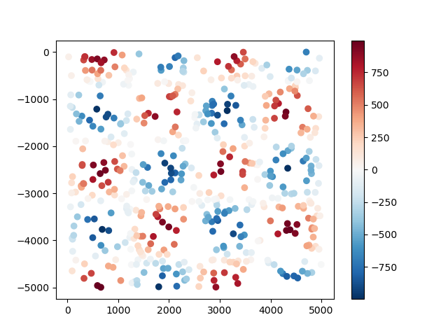
As an example, let’s generate some synthetic data using verde.datasets.CheckerBoard:

data = vd.datasets.CheckerBoard().scatter(size=500, random_state=0)
print(data.head())

Out:

      northing      easting     scalars
0 -3448.095870  2744.067520 -417.745960
1 -3134.825681  3575.946832  -10.460197
2 -2375.147789  3013.816880  914.277006
3 -1247.024885  2724.415915 -534.571829
4 -3332.462671  2118.273997  407.865799

The data are random points taken from a checkerboard function and returned to us in a pandas.DataFrame:

import matplotlib.pyplot as plt

plt.figure()
plt.scatter(data.easting, data.northing, c=data.scalars, cmap="RdBu_r")
plt.colorbar()
plt.show()

Now we can use the bi-harmonic spline method [Sandwell1987] to fit this data. First, we create a new verde.Spline:

spline = vd.Spline()
# Printing a gridder shows the class and all of it's configuration options.
print(spline)

Out:

Spline()

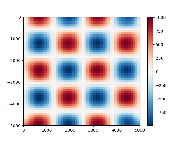
Before we can use the spline, we need to fit it to our synthetic data. After that, we can use the spline to predict values anywhere:

spline.fit((data.easting, data.northing), data.scalars)

# Generate coordinates for a regular grid with 100 m grid spacing (assuming coordinates
# are in meters).
grid_coords = vd.grid_coordinates(region=(0, 5000, -5000, 0), spacing=100)
gridded_scalars = spline.predict(grid_coords)

plt.figure()
plt.pcolormesh(grid_coords[0], grid_coords[1], gridded_scalars, cmap="RdBu_r")
plt.colorbar()
plt.show()

Out:

/home/runner/work/verde/verde/tutorials/overview.py:102: MatplotlibDeprecationWarning: shading='flat' when X and Y have the same dimensions as C is deprecated since 3.3.  Either specify the corners of the quadrilaterals with X and Y, or pass shading='auto', 'nearest' or 'gouraud', or set rcParams['pcolor.shading'].  This will become an error two minor releases later.
  plt.pcolormesh(grid_coords[0], grid_coords[1], gridded_scalars, cmap="RdBu_r")

We can compare our predictions with the true values for the checkerboard function using the score method to calculate the R² coefficient of determination.

true_values = vd.datasets.CheckerBoard().predict(grid_coords)
print(spline.score(grid_coords, true_values))

Out:

0.9950450871662091

Generating grids and profiles

A more convenient way of generating grids is through the grid method. It will automatically generate coordinates and output an xarray.Dataset.

grid = spline.grid(spacing=30)
print(grid)

Out:

<xarray.Dataset>
Dimensions:   (easting: 167, northing: 168)
Coordinates:
  * easting   (easting) float64 23.48 53.42 83.37 ... 4.964e+03 4.994e+03
  * northing  (northing) float64 -4.997e+03 -4.967e+03 ... -30.88 -0.9571
Data variables:
    scalars   (northing, easting) float64 495.6 521.3 549.0 ... -184.7 -139.6
Attributes:
    metadata:  Generated by Spline()

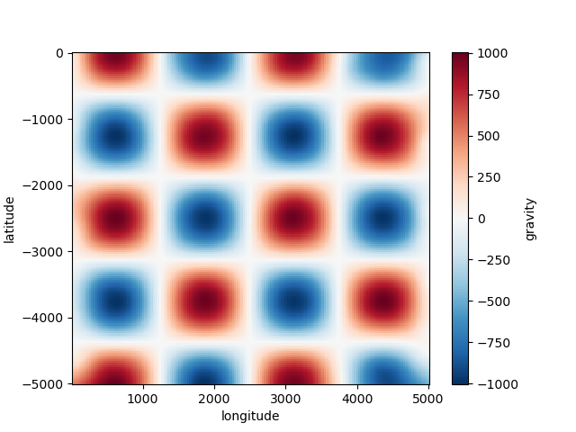
grid uses default names for the coordinates (“easting” and “northing”) and data variables (“scalars”). You can overwrite these names by setting the dims and data_names arguments.

grid = spline.grid(spacing=30, dims=["latitude", "longitude"], data_names="gravity")
print(grid)

plt.figure()
grid.gravity.plot.pcolormesh()
plt.show()

Out:

<xarray.Dataset>
Dimensions:    (latitude: 168, longitude: 167)
Coordinates:
  * longitude  (longitude) float64 23.48 53.42 83.37 ... 4.964e+03 4.994e+03
  * latitude   (latitude) float64 -4.997e+03 -4.967e+03 ... -30.88 -0.9571
Data variables:
    gravity    (latitude, longitude) float64 495.6 521.3 549.0 ... -184.7 -139.6
Attributes:
    metadata:  Generated by Spline()

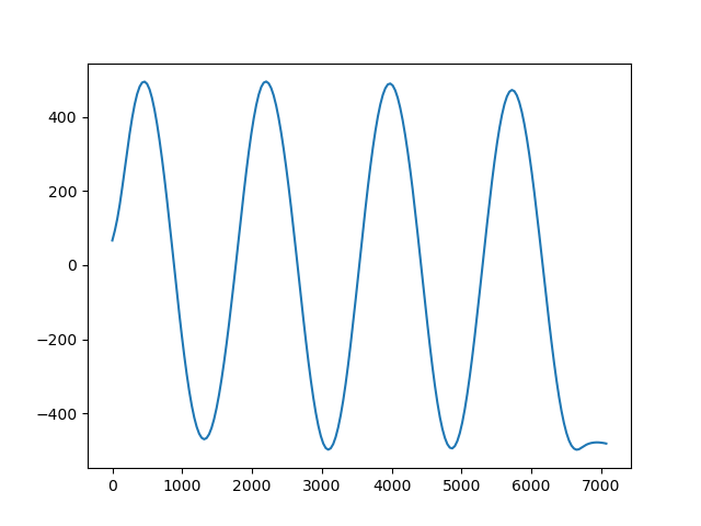
Gridders can also be used to interpolate data on a straight line between two points using the profile method. The profile data are returned as a pandas.DataFrame.

prof = spline.profile(point1=(0, 0), point2=(5000, -5000), size=200)
print(prof.head())

plt.figure()
plt.plot(prof.distance, prof.scalars, "-")
plt.show()

Out:

     northing     easting    distance     scalars
0    0.000000    0.000000    0.000000   66.785376
1  -25.125628   25.125628   35.533004   92.895113
2  -50.251256   50.251256   71.066008  124.644012
3  -75.376884   75.376884  106.599012  163.870392
4 -100.502513  100.502513  142.132016  209.836541

Wrap up

This covers the basics of using Verde. Most use cases and examples in the documentation will involve some variation of the following workflow:

1. Load data (coordinates and data values)

2. Create a gridder

3. Fit the gridder to the data

4. Predict new values (using predict or grid)