Note
Click here to download the full example code
Geographic Coordinates
Most gridders and processing methods in Verde operate under the assumption that the data coordinates are Cartesian. To process data in geographic (longitude and latitude) coordinates, we must first project them. There are different ways of doing this in Python but most of them rely on the PROJ library. We’ll use pyproj to access PROJ directly and handle the projection operations.
import pyproj
import numpy as np
import matplotlib.pyplot as plt
import cartopy.crs as ccrs
import verde as vd
With pyproj, we can create functions that will project our coordinates to and from different coordinate systems. For our Baja California bathymetry data, we’ll use a Mercator projection.
data = vd.datasets.fetch_baja_bathymetry()
# We're choosing the latitude of true scale as the mean latitude of our dataset.
projection = pyproj.Proj(proj="merc", lat_ts=data.latitude.mean())
The Proj object is a callable (meaning that it behaves like a function) that will take longitude and latitude and return easting and northing coordinates.
# pyproj doesn't play well with Pandas so we need to convert to numpy arrays
proj_coords = projection(data.longitude.values, data.latitude.values)
print(proj_coords)
Out:
(array([-11749316.65303045, -11748999.90777981, -11748682.14077028, ...,
       -11749178.71558258, -11749531.2223938 , -11749882.70744612]), array([2905766.05183735, 2905457.83817751, 2905148.48639437, ...,
       2579612.89349502, 2580017.48641078, 2580422.09116872]))
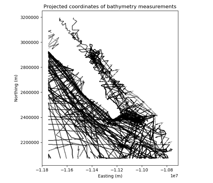
We can plot our projected coordinates using matplotlib.
plt.figure(figsize=(7, 6))
plt.title("Projected coordinates of bathymetry measurements")
# Plot the bathymetry data locations as black dots
plt.plot(proj_coords[0], proj_coords[1], ".k", markersize=0.5)
plt.xlabel("Easting (m)")
plt.ylabel("Northing (m)")
plt.gca().set_aspect("equal")
plt.tight_layout()
plt.show()
Cartesian grids
Now we can use verde.BlockReduce and verde.Spline on our projected
coordinates. We’ll specify the desired grid spacing as degrees and convert it to
Cartesian using the 1 degree approx. 111 km rule-of-thumb.
spacing = 10 / 60
reducer = vd.BlockReduce(np.median, spacing=spacing * 111e3)
filter_coords, filter_bathy = reducer.filter(proj_coords, data.bathymetry_m)
spline = vd.Spline().fit(filter_coords, filter_bathy)
If we now call verde.Spline.grid we’ll get back a grid evenly spaced in
projected Cartesian coordinates.
grid = spline.grid(spacing=spacing * 111e3, data_names=["bathymetry"])
print("Cartesian grid:")
print(grid)
Out:
Cartesian grid:
<xarray.Dataset>
Dimensions:     (easting: 54, northing: 61)
Coordinates:
  * easting     (easting) float64 -1.175e+07 -1.173e+07 -1.171e+07 ...
  * northing    (northing) float64 2.074e+06 2.093e+06 2.112e+06 2.13e+06 ...
Data variables:
    bathymetry  (northing, easting) float64 -3.635e+03 -3.727e+03 -3.783e+03 ...
Attributes:
    metadata:  Generated by Spline(damping=None, engine='auto',\n    force_co...
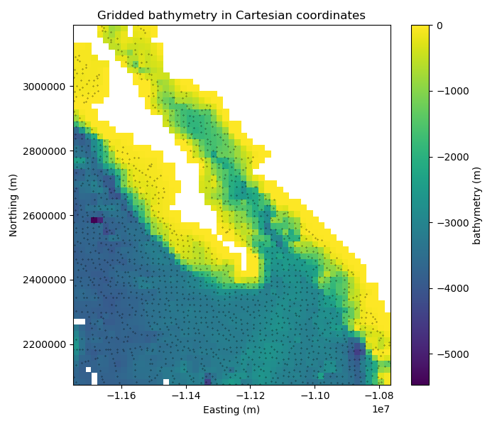
We’ll mask our grid using verde.distance_mask to get rid of all the spurious
solutions far away from the data points.
grid = vd.distance_mask(proj_coords, maxdist=30e3, grid=grid)

plt.figure(figsize=(7, 6))
plt.title("Gridded bathymetry in Cartesian coordinates")
plt.pcolormesh(grid.easting, grid.northing, grid.bathymetry, cmap="viridis", vmax=0)
plt.colorbar().set_label("bathymetry (m)")
plt.plot(filter_coords[0], filter_coords[1], ".k", markersize=0.5)
plt.xlabel("Easting (m)")
plt.ylabel("Northing (m)")
plt.gca().set_aspect("equal")
plt.tight_layout()
plt.show()
Geographic grids
The Cartesian grid that we generated won’t be evenly spaced if we convert the
coordinates back to geographic latitude and longitude. Verde gridders allow you to
generate an evenly spaced grid in geographic coordinates through the projection
argument of the grid method.
By providing a projection function (like our pyproj projection object), Verde will
generate coordinates for a regular grid and then pass them through the projection
function before predicting data values. This way, you can generate a grid in a
coordinate system other than the one you used to fit the spline.
# Get the geographic bounding region of the data
region = vd.get_region((data.longitude, data.latitude))
print("Data region in degrees:", region)

# Specify the region and spacing in degrees and a projection function
grid_geo = spline.grid(
    region=region,
    spacing=spacing,
    projection=projection,
    dims=["latitude", "longitude"],
    data_names=["bathymetry"],
)
print("Geographic grid:")
print(grid_geo)
Out:
Data region in degrees: (245.0, 254.705, 20.0, 29.99131)
Geographic grid:
<xarray.Dataset>
Dimensions:     (latitude: 61, longitude: 59)
Coordinates:
  * longitude   (longitude) float64 245.0 245.2 245.3 245.5 245.7 245.8 ...
  * latitude    (latitude) float64 20.0 20.17 20.33 20.5 20.67 20.83 21.0 ...
Data variables:
    bathymetry  (latitude, longitude) float64 -3.621e+03 -3.709e+03 ...
Attributes:
    metadata:  Generated by Spline(damping=None, engine='auto',\n    force_co...
Notice that grid has longitude and latitude coordinates and slightly different number of points than the Cartesian grid.
The verde.distance_mask function also supports the projection argument and
will project the coordinates before calculating distances.
grid_geo = vd.distance_mask(
    (data.longitude, data.latitude), maxdist=30e3, grid=grid_geo, projection=projection
)
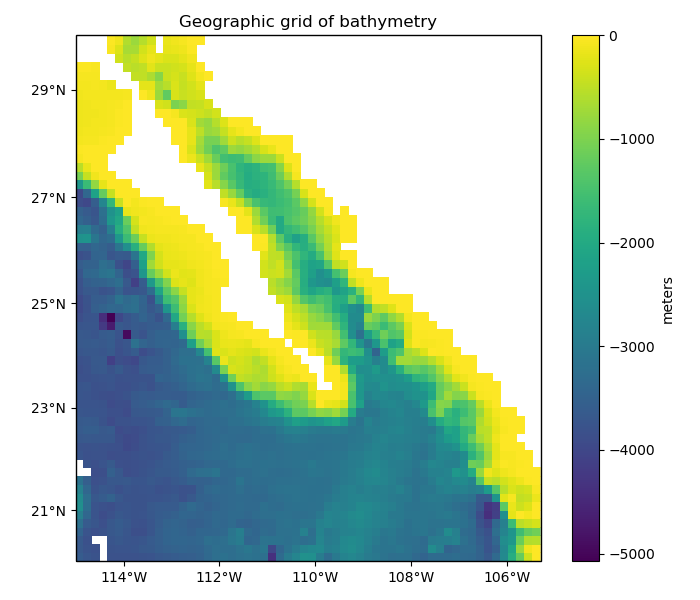
Now we can use the Cartopy library to plot our geographic grid.
plt.figure(figsize=(7, 6))
ax = plt.axes(projection=ccrs.Mercator())
ax.set_title("Geographic grid of bathymetry")
pc = ax.pcolormesh(
    grid_geo.longitude,
    grid_geo.latitude,
    grid_geo.bathymetry,
    transform=ccrs.PlateCarree(),
    vmax=0,
    zorder=-1,
)
plt.colorbar(pc).set_label("meters")
vd.datasets.setup_baja_bathymetry_map(ax, land=None)
plt.tight_layout()
plt.show()
Total running time of the script: ( 0 minutes 8.531 seconds)