Chaining operations

The verde.Chain class allows us to created gridders that perform multiple operations on data. Each step in the chain filters the input and passes the result along to the next step. For gridders and trend estimators, filtering means fitting the model and passing along the residuals (input data minus predicted data). When predicting data, the predictions of each step are added together. Other operations, like verde.BlockReduce and verde.BlockMean change the input data values and the coordinates as well but don’t impact the predictions directly.

For example, say we want to decimate some data, calculate a polynomial trend, and fit a gridder on the residual values (not the trend), but then make a grid of the full data values (trend included). This is useful because decimation is common and many gridders can’t handle trends in data.

Out:

Chained estimator: Chain(steps=[('trend', Trend(degree=2)), ('reduce', BlockReduce(adjust='spacing', center_coordinates=False,
      reduction=<function mean at 0x14ecd05ca2f0>, region=None,
      spacing=925.0)), ('spline', Spline(damping=1e-08, engine='auto', mindist=50000.0, region=None, shape=None,
    spacing=None))])

Trend grid:
<xarray.Dataset>
Dimensions:   (easting: 101, northing: 101)
Coordinates:
  * easting   (easting) float64 -4.391e+06 -4.391e+06 -4.39e+06 -4.389e+06 ...
  * northing  (northing) float64 -2.366e+06 -2.366e+06 -2.365e+06 -2.365e+06 ...
Data variables:
    scalars   (northing, easting) float64 91.02 92.92 94.83 96.74 98.65 ...
Attributes:
    metadata:  Generated by Trend(degree=2)

Residual grid:
<xarray.Dataset>
Dimensions:   (easting: 101, northing: 101)
Coordinates:
  * easting   (easting) float64 -4.391e+06 -4.391e+06 -4.39e+06 -4.389e+06 ...
  * northing  (northing) float64 -2.366e+06 -2.365e+06 -2.365e+06 -2.364e+06 ...
Data variables:
    scalars   (northing, easting) float64 34.88 35.11 30.96 22.31 25.44 ...
Attributes:
    metadata:  Generated by Spline(damping=1e-08, engine='auto', mindist=5000...

Chained geographic grid:
<xarray.Dataset>
Dimensions:              (latitude: 61, longitude: 73)
Coordinates:
  * longitude            (longitude) float64 -42.6 -42.59 -42.58 -42.57 ...
  * latitude             (latitude) float64 -22.5 -22.49 -22.48 -22.48 ...
Data variables:
    total_field_anomaly  (latitude, longitude) float64 124.8 126.1 119.6 ...
Attributes:
    metadata:  Generated by Chain(steps=[('trend', Trend(degree=2)), ('reduce...

import numpy as np
import matplotlib.pyplot as plt
import cartopy.crs as ccrs
import pyproj
import verde as vd

# Load the Rio de Janeiro total field magnetic anomaly data
data = vd.datasets.fetch_rio_magnetic()
region = vd.get_region((data.longitude, data.latitude))

# Create a projection for the data using pyproj so that we can use it as input for the
# gridder. We'll set the latitude of true scale to the mean latitude of the data.
projection = pyproj.Proj(proj="merc", lat_ts=data.latitude.mean())

# Create a chain that fits a 2nd degree trend, decimates the residuals using a blocked
# mean to avoid aliasing, and then fits a standard gridder to the residuals. The spacing
# for the blocked mean will be 0.5 arc-minutes (approximately converted to meters).
spacing = 0.5 / 60
chain = vd.Chain(
    [
        ("trend", vd.Trend(degree=2)),
        ("reduce", vd.BlockReduce(np.mean, spacing * 111e3)),
        ("spline", vd.Spline(damping=1e-8, mindist=50e3)),
    ]
)
print("Chained estimator:", chain)
# Calling 'fit' will automatically run the data through the chain
chain.fit(
    projection(data.longitude.values, data.latitude.values), data.total_field_anomaly_nt
)

# Each component of the chain can be accessed separately using the 'named_steps'
# attribute
grid_trend = chain.named_steps["trend"].grid()
print("\nTrend grid:")
print(grid_trend)

grid_residual = chain.named_steps["spline"].grid()
print("\nResidual grid:")
print(grid_residual)

# Chain.grid will use both the trend and the gridder to predict values. We'll use the
# 'projection' keyword to generate a geographic grid instead of Cartesian
grid = chain.grid(
    region=region,
    spacing=spacing,
    projection=projection,
    dims=["latitude", "longitude"],
    data_names=["total_field_anomaly"],
)
print("\nChained geographic grid:")
print(grid)

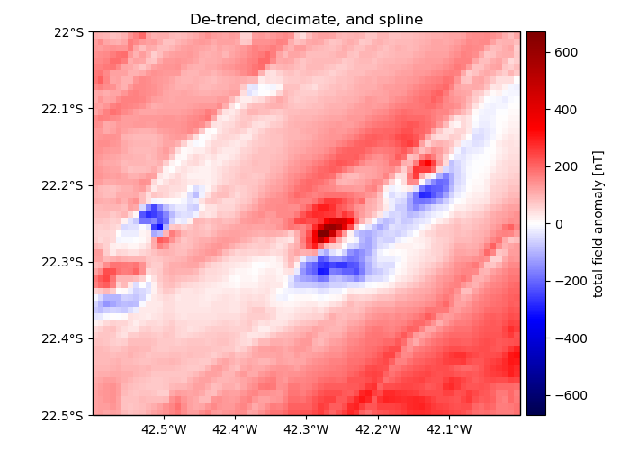
# We'll plot only the chained grid on a Mercator map
plt.figure(figsize=(7, 5))
crs = ccrs.PlateCarree()
ax = plt.axes(projection=ccrs.Mercator())
ax.set_title("De-trend, decimate, and spline")
maxabs = vd.maxabs(grid.total_field_anomaly)
pc = ax.pcolormesh(
    grid.longitude,
    grid.latitude,
    grid.total_field_anomaly,
    transform=crs,
    cmap="seismic",
    vmin=-maxabs,
    vmax=maxabs,
)
plt.colorbar(pc, pad=0.01).set_label("total field anomaly [nT]")
# Set the proper ticks for a Cartopy map
vd.datasets.setup_rio_magnetic_map(ax)
plt.tight_layout()
plt.show()

Total running time of the script: ( 0 minutes 6.372 seconds)