harmonica.isostasy_airy
-
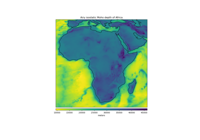
harmonica.isostasy_airy(topography, density_crust=2800.0, density_mantle=3300.0, density_water=1000.0, reference_depth=30000.0)[source]¶ Calculate the isostatic Moho depth from topography using Airy’s hypothesis.
According to the Airy hypothesis of isostasy, topography above sea level is supported by a thickening of the crust (a root) while oceanic basins are supported by a thinning of the crust (an anti-root). This assumption is usually

Schematic of isostatic compensation following the Airy hypothesis.
The relationship between the topographic/bathymetric heights (\(h\)) and the root thickness (\(r\)) is governed by mass balance relations and can be found in classic textbooks like [TurcotteSchubert2014] and [Hofmann-WellenhofMoritz2006].
On the continents (positive topographic heights):
\[r = \frac{\rho_{c}}{\rho_m - \rho_{c}} h\]while on the oceans (negative topographic heights):
\[r = \frac{\rho_{c} - \rho_w}{\rho_m - \rho_{c}} h\]in which \(h\) is the topography/bathymetry, \(\rho_m\) is the density of the mantle, \(\rho_w\) is the density of the water, and \(\rho_{c}\) is the density of the crust.
The computed root thicknesses will be added to the given reference Moho depth (\(H\)) to arrive at the isostatic Moho depth. Use
reference_depth=0if you want the values of the root thicknesses instead.- Parameters
topography (array or
xarray.DataArray) – Topography height and bathymetry depth in meters. It is usually prudent to use floating point values instead of integers to avoid integer division errors.density_crust (float) – Density of the crust in \(kg/m^3\).
density_mantle (float) – Mantle density in \(kg/m^3\).
density_water (float) – Water density in \(kg/m^3\).
reference_depth (float) – The reference Moho depth (\(H\)) in meters.
- Returns
moho_depth (array or
xarray.DataArray) – The isostatic Moho depth in meters.