Point Masses in Cartesian Coordinates

The simplest geometry used to compute gravitational fields are point masses. Although modelling geologic structures with point masses can be challenging, they are very useful for other purposes: creating synthetic models, solving inverse problems, generating equivalent sources for interpolation, etc. The gravitational fields generated by point masses can be quickly computed either in Cartesian or in geocentric spherical coordinate systems. We will compute the gravitational acceleration generated by a set of point masses on a computation grid given in Cartesian coordinates using the harmonica.point_mass_gravity function.

Out:

[[ 0.00181314  0.00190983  0.00200888 ... -0.00328218 -0.0032428
  -0.00320183]
 [ 0.00196785  0.00207626  0.00218766 ... -0.0034324  -0.00338955
  -0.00334507]
 [ 0.0021343   0.00225579  0.00238107 ... -0.00359128 -0.00354465
  -0.00349633]
 ...
 [-0.0014489  -0.00151296 -0.0015806  ... -0.01802268 -0.01727698
  -0.01655213]
 [-0.00144777 -0.00151078 -0.00157723 ... -0.01697132 -0.0162955
  -0.01563681]
 [-0.00144484 -0.00150675 -0.00157197 ... -0.01599028 -0.01537726
  -0.01477824]]
/home/runner/work/harmonica/harmonica/examples/forward/point_mass.py:62: UserWarning: FixedFormatter should only be used together with FixedLocator
  ax.set_xticklabels(ax.get_xticks() * 1e-3)
/home/runner/work/harmonica/harmonica/examples/forward/point_mass.py:63: UserWarning: FixedFormatter should only be used together with FixedLocator
  ax.set_yticklabels(ax.get_yticks() * 1e-3)

import harmonica as hm
import verde as vd
import matplotlib.pyplot as plt
import matplotlib.ticker


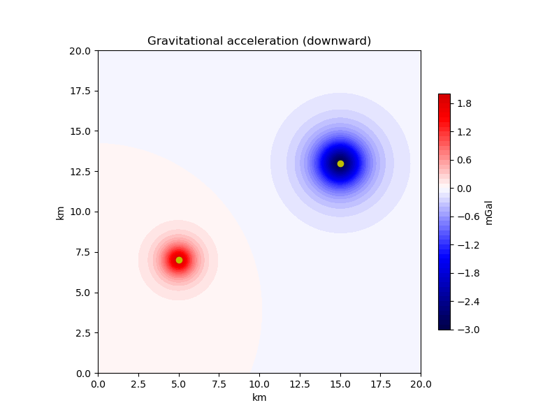
# Define the coordinates for two point masses
easting = [5e3, 15e3]
northing = [7e3, 13e3]
# The vertical coordinate is positive upward so negative numbers represent
# depth
upward = [-0.5e3, -1e3]
points = [easting, northing, upward]
# We're using "negative" masses to represent a "mass deficit" since we assume
# measurements are gravity disturbances, not actual gravity values.
masses = [3e11, -10e11]

# Define computation points on a grid at 500m above the ground
coordinates = vd.grid_coordinates(
    region=[0, 20e3, 0, 20e3], shape=(100, 100), extra_coords=500
)

# Compute the downward component of the gravitational acceleration
gravity = hm.point_mass_gravity(
    coordinates, points, masses, field="g_z", coordinate_system="cartesian"
)
print(gravity)

# Plot the results on a map
fig, ax = plt.subplots(figsize=(8, 6))
ax.set_aspect("equal")
# Get the maximum absolute value so we can center the colorbar on zero
maxabs = vd.maxabs(gravity)
img = ax.contourf(
    *coordinates[:2], gravity, 60, vmin=-maxabs, vmax=maxabs, cmap="seismic"
)
plt.colorbar(img, ax=ax, pad=0.04, shrink=0.73, label="mGal")
# Plot the point mass locations
ax.plot(easting, northing, "oy")
ax.set_title("Gravitational acceleration (downward)")
# Convert axes units to km
ax.set_xticklabels(ax.get_xticks() * 1e-3)
ax.set_yticklabels(ax.get_yticks() * 1e-3)
ax.set_xlabel("km")
ax.set_ylabel("km")
plt.show()